Quick Response to Fangraphs War Article

A response to this article on Fangraphs.

WAR has an R^2 of .83, but what does that really mean? Some context (all stats from ESPN.com):

ALwins ALera ALba ALops ALrbi

ALwins 1.000 -0.642 0.588 0.704 0.672

That is how American League wins correlates (little "r" not R^2) with ERA, Batting Average, OPS, and RBI. And the NL:

NLwins NLera NLba NLops NLrbi

NLwins 1.000 -0.751 0.369 0.503 0.572

I made three linear models for each league to find the R^2 of wins versus ERA and BA, ERA and RBI, and ERA and RBI. The R^2 values are .84, .86, and .87 respectively for the AL. For the NL .61, .82, and .81. Below are the print outs from R.

Call:

lm(formula = ALwins ~ ALera + ALba)

Residuals:

Min 1Q Median 3Q Max

-7.6862 -2.7943 -0.7403 1.9202 9.0998

Coefficients:

Estimate Std. Error t value Pr(>|t|)

(Intercept) -49.532 46.485 -1.066 0.309461

ALera -24.762 4.224 -5.862 0.000109 ***

ALba 907.270 166.522 5.448 0.000201 ***

---

Signif. codes: 0 ‘***’ 0.001 ‘**’ 0.01 ‘*’ 0.05 ‘.’ 0.1 ‘ ’ 1

Residual standard error: 5.265 on 11 degrees of freedom

Multiple R-squared: 0.8414, Adjusted R-squared: 0.8126

F-statistic: 29.18 on 2 and 11 DF, p-value: 3.995e-05

> summary(al2)

Call:

lm(formula = ALwins ~ ALera + ALrbi)

Residuals:

Min 1Q Median 3Q Max

-8.888 -2.575 1.766 3.284 5.192

Coefficients:

Estimate Std. Error t value Pr(>|t|)

(Intercept) 96.20702 22.96652 4.189 0.001513 **

ALera -22.33402 3.96918 -5.627 0.000154 ***

ALrbi 0.11425 0.01941 5.885 0.000105 ***

---

Signif. codes: 0 ‘***’ 0.001 ‘**’ 0.01 ‘*’ 0.05 ‘.’ 0.1 ‘ ’ 1

Residual standard error: 4.971 on 11 degrees of freedom

Multiple R-squared: 0.8586, Adjusted R-squared: 0.8329

F-statistic: 33.4 on 2 and 11 DF, p-value: 2.124e-05

> summary(al3)

Call:

lm(formula = ALwins ~ ALera + ALops)

Residuals:

Min 1Q Median 3Q Max

-8.8988 -2.1200 0.6058 2.9829 8.0973

Coefficients:

Estimate Std. Error t value Pr(>|t|)

(Intercept) -6.139 34.441 -0.178 0.861764

ALera -21.489 3.783 -5.681 0.000142 ***

ALops 240.741 38.383 6.272 6.07e-05 ***

---

Signif. codes: 0 ‘***’ 0.001 ‘**’ 0.01 ‘*’ 0.05 ‘.’ 0.1 ‘ ’ 1

Residual standard error: 4.734 on 11 degrees of freedom

Multiple R-squared: 0.8718, Adjusted R-squared: 0.8485

F-statistic: 37.41 on 2 and 11 DF, p-value: 1.239e-05

summary(nl1)

Call:

lm(formula = NLwins ~ NLera + NLba)

Residuals:

Min 1Q Median 3Q Max

-9.467 -4.923 -1.258 3.634 12.506

Coefficients:

Estimate Std. Error t value Pr(>|t|)

(Intercept) 69.111 70.851 0.975 0.34714

NLera -16.635 4.173 -3.986 0.00155 **

NLba 312.338 251.322 1.243 0.23590

---

Signif. codes: 0 ‘***’ 0.001 ‘**’ 0.01 ‘*’ 0.05 ‘.’ 0.1 ‘ ’ 1

Residual standard error: 7.43 on 13 degrees of freedom

Multiple R-squared: 0.6113, Adjusted R-squared: 0.5515

F-statistic: 10.22 on 2 and 13 DF, p-value: 0.002150

> summary(nl2)

Call:

lm(formula = NLwins ~ NLera + NLrbi)

Residuals:

Min 1Q Median 3Q Max

-7.950 -3.843 1.426 3.937 5.915

Coefficients:

Estimate Std. Error t value Pr(>|t|)

(Intercept) 85.42980 19.82645 4.309 0.000849 ***

NLera -16.63429 2.77925 -5.985 4.55e-05 ***

NLrbi 0.09444 0.02190 4.311 0.000845 ***

---

Signif. codes: 0 ‘***’ 0.001 ‘**’ 0.01 ‘*’ 0.05 ‘.’ 0.1 ‘ ’ 1

Residual standard error: 5.042 on 13 degrees of freedom

Multiple R-squared: 0.821, Adjusted R-squared: 0.7935

F-statistic: 29.82 on 2 and 13 DF, p-value: 1.39e-05

> summary(nl3)

Call:

lm(formula = NLwins ~ NLera + NLops)

Residuals:

Min 1Q Median 3Q Max

-7.792 -3.753 1.456 4.205 5.731

Coefficients:

Estimate Std. Error t value Pr(>|t|)

(Intercept) 2.526 39.070 0.065 0.94944

NLera -17.588 2.853 -6.164 3.41e-05 ***

NLops 204.851 50.095 4.089 0.00128 **

---

Signif. codes: 0 ‘***’ 0.001 ‘**’ 0.01 ‘*’ 0.05 ‘.’ 0.1 ‘ ’ 1

Residual standard error: 5.198 on 13 degrees of freedom

Multiple R-squared: 0.8098, Adjusted R-squared: 0.7805

F-statistic: 27.67 on 2 and 13 DF, p-value: 2.065e-05

Yet Another Way to Look at Free Throw Percentage

John Branch wrote an article in the New York Times noting that in the past 50 years, Free Throw Percentage (FT%) has not improved in the NBA. The Freakonomics blog posted a follow up to this article that suggested that free throw percentage among the best Free Throw (FT) shooters has improved during that period. Unfortunately, I read this post and wasted the best weather of the year fooling around on R rather than going outside and getting sunburnt.

Ashley Smart, the person who supplied the data and analysis the blog post is based on, seems intelligent and probably knows more about stats than I do. The data she has for her analysis is deeply flawed. The biggest mistake she made was getting the data from N.B.A. Encyclopedia. The place for NBA data is Basketball Reference. You can download several spreadsheets of NBA data stretching back to 1946. As several commentators noted, Ms. Smart's other mistake is not controlling for the number of players.

That said there are two major flaws in Ms. Smart's analysis:

1. The NBA Encyclopedia is arbitrary and inconsisent. The data collectors changed their standards on who qualified as a top 20 FT shooter 14 times between 1950 and 2007. The biggest supposed gain in FT% in Ms. Smart's study occurs between the 1972 and 1973 seasons when qualification standards go from 350 Free Throw Attempts (FTA) to 160 FTA. 
2. The study does not account for the number of players in the league. Of course the top 20 players in the league now are going to have a better FT% than those in 1950. In 1950 there were 135 players, in 2007 595 players. If I took a group of 100 random people and made them shoot a bunch of Free Throws and then took a group of 500 people and made them shoot a bunch of Free Throws which group do you think would have the best average among the top 20 Free Throw shooters? 

I corrected the first problem by getting my data from Basketball Reference. Anyone who had 100 FTA qualified for my analysis. Let us take a look at the Top Twenty players in FT% versus the number of players in the league.

And a look at the number of players by year:

For what it's worth, there is an R^2 value of .82 for Number of Players vs. Top Twenty FT% and an R^2 value of .76 for Year vs. Top Twenty FT% for fitted linear models. The two models have too much serial correlation to be taken seriously. Year and Number of Players has a .93 correlation value.

A hopefully correct method for examining the best FT shooters is to look at the Top Tenth Percentile of FT% for each year:

There appears to be a slight increase in the FT% of the top tenth percentile but once again there is serial correlation. A Durbin Watson test confirms this; D-W Statistic of .978--anything below 1.38 for this sample size is suspicious--with a p-value of 0 and estimated rho value of .51. I did a basic transformation of the Year (X) and Top Tenth Percentile FT% (Y) variables:

Ytransformed = Yi+1 - rho*Yi 

Xtransformed = Xi+1 - rho*Xi

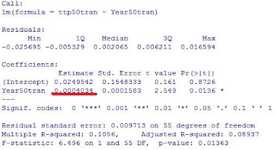
I then fit a new model of Xtransformed verus Ytransformed. The D-W statistic was 1.89 with a p value of .58 and an estimated rho of .05, thus removing the serial correlation. A summary of this model:

With such a poor fitting model (R^2 of .1056) the data does not really explain anything. If I were going to make an inference I would point out the underlined value of .0004034 (b1). The regression coeffecient for X for the transformed model will remain the same when the model is tranformed back to Y = b1*X + b0. So over the 57 years of data, 57*b1 = 2.3% increase in the Top Tenth Percentile FT%. This is really stretching the model but there may be a slight increase (2.3% over 57 years) among the best FT shooters.