More Memory Game

This post is an attempt to answer the question I posed in a prior post about the Memory Game. If you are not familiar with the Memory Game, you can read that post to get familiar with the rules and terminology. The question:

With the second part of your turn, if you do not have a 100% chance of getting a pair is it better to flip an already known tile or try to flip an unknown tile?

As I explained in my prior post on Memory, there are two ways to score. The first method of scoring is to flip over your first tile and already know the position of its match on the board. The second method of scoring is to flip over your first tile, not know the position of its match, and then randomly guess and find its match. My question asks should you forgo the second method of scoring pairs? 

Memory Game

In the seventh episode of this season (22nd) of Survivor, two contestants played the Memory Game to see who would remain on the show. In the Memory Game you score points by flipping over pairs of the same card. Whoever identifies the most pairs wins. The Survivor version had 20 tiles (10 unique pairs) laid face down. The contestants took turns flipping over two tiles per turn. If you flipped over identical tiles (a pair) you received a point and those two tiles were removed from the game. If the contestant flipped over non-identical tiles, the tiles were returned to their face down position. The players alternated turns regardless of whether they scored a pair or not. First to get five pairs won the game. Watching the game, I had two questions:

1. Is it better to go first or second?
2. With the second part of your turn, if you do not have a 100% chance of getting a pair is it better to flip an already known tile or try to flip an unknown tile?

NBA Salary Commitments

As I sit around killing time until I can play some pick up basketball at the park, I'm taking a look at the salary data available at HoopsHype.com.  NBA salaries amuse.  Every year we get to see the winner's curse in action.  They gave how much to Joe Johnson?  Why on earth would you sign Hedo Turkoglu to a five year deal (and how the heck was he traded twice within the first 18 months of his contract)?  I took a look at each team and made some tables and graphs of each team's salary commitment.

More Fangraphs.com Org Rankings

To see the data in spreadsheet form, click here. You can see how teams changed in versus last years ranking and where they scored in each of the four component categories. Toronto, San Fransisco, Cincinatti, and the White Sox moved up 10 or more places while Milwaukee, Seattle, Cleveland, and Arizona were the big downgrades. I didn't like how Future Talent was compiled and have some reservations about Financial Resources  (perhaps a topic for another post).

Fangraphs.com Organization Rankings -- Star Plots

Fangraphs.com has an annual series of posts where they rank each Major League Baseball organization on the following criteria: Present Talent (30%), Financial Resources (30%), Baseball Operations (25%), and Future Talent (15%). The writers grade each team in each of the categories probably on a scale of 1-100 (I believe; no ranking is below 62 or above 95). I took the rankings for each category and made some star plots.

The Challenge: Cutthroat

After two episodes the MTV reality show The Challenge: Cutthroat has not had much to analyze strategically. The only major choices faced so far have been picking the teams and choosing who gets sent into the elimination round.

Bill Simmons and the NFC West

In his weekly football column, Bill Simmons of ESPN.com harshly criticizes the NFC West. His main point of evidence is the NFC's west record since 2002 (go-go arbitrary end points). He posts this table in his article:

Aging Curves in Basketball

The NBA offseason raised a few questions. In order to answer these questions I need to do a little research and figure out a few things. One of these things is an aging curve for basketball players. What is their prime? What rate do they decline after that prime? Luckily this question has been asked and answered in baseball so I can use their methodology and apply it to basketball.

For data, I went to www.basketball-reference.com and pulled the advanced data for players from the 2000-2001 season through the 2009-2010 season (the seasons from the last collective bargaining agreement). My methodology follows the work of TangoTiger and MGL, particularly this article written by MGL. I will try to briefly summarize the methodology. MGL offers a much clearer explanation so I recommend reading that article first.

The World Cup Approaches...

Another World Cup tradition: players complaining about the new ball. The Adidas Jabulani replaces the much maligned 2006 Teamgeist and the hated 2002 Fevernova. Goalkeepers complained about the 1994 Questra ball and I'm sure soccer players wished many unkind things towards the 1998 Tricolore ball but I can't find a link. I'm not sure why but I find the sky-is-falling stories about the new balls amusing.

Fresh Meat II: Episode 7

Continuing my strange fascination with the MTV show Fresh Meat II, here's a post about the latest episode. Wes's coalition officially reached its end as the two remaining teams in it where forced into the elimination challenge. Wes's team lost and left the game. We are left with 6 teams. 4 eams are in Kenny's alliance and 2 are on the outskirts. The last 4 teams go to the finals where they compete for cash money. 1st place in the final challenge wins $200k, 2nd place $60k, 3rd place $40k, and 4th place receives nothing. The goal is to not only make it to the finals, but to maximize your expected winnings in the finals. Strategically, how should the six remaining teams behave to optimize their expected payout?

The Challenge: Fresh Meat II Episode 6

A few weeks ago I wrote a post saying that Kenny's alliance had basically no chance to retake the majority (0.2%). The Kenny's alliance was down 7 teams to 3. The alliance would have to win 4 reward challenges and 3 elimination challenges in order to take back the majority. 3 reward challenge victories and 3 elimination challenge victories later, Kenny's alliance has seized control of the game and is in a dominant position. What happened? Why was I so wrong in underestimating the chances of Kenny's alliance?

Fresh Meat II: The Challenge Episode #4

My earlier posts on the MTV reality show Fresh Meat II: The Challenge recommended two strategies for the competing factions in the show: one side should tighten the bounds in its group and keep loyalty strong while the other side should use the threat throwing a team into the elimination challenge as a way to get teams to defect to their faction. However the factions got the strategies backwards. I recommended Kenny's alliance use the threat of being sent into the elimination challenge to get someone to defect to his alliance. Wes's coalition had the superior numbers. It was in Wes's coalition's best interests to keep loyalty strong within the group. Instead Kenny let someone in his alliance choose who was going into the elimination challenge, thus trying to boost loyalty withing the group while Wes's coalition used the threat of being thrown into the elimination round to get a team to defect to his coalition.

NBA #1 Seeds that Struggle in the First Round

A post on Hoops Analyst talks about the Los Angeles Lakers - Oklahoma Thunder NBA playoff first round series. The Lakers are the highly rated #1 seed and the Thunder are the lowest rated #8 seed. The two teams are playing a best-of-seven series. The author asks if a #1 seed that is struggling against a #8 seed is "a bad indicator for their success in the playoffs"? The post then looks at each of the #1 seeds that struggled against #8 seeds and concludes "I would venture that there is little correlation between a round one struggle and overall team weakness." What does the data say?

The Challenge: Fresh Meat II Wes's Coalition

With Wes's coalition in such a dominate position, the 7 teams in it have to start moving beyond the threat of Kenny's alliance (3 teams) and strategizing  for the end game. In particular two things: avoiding the elimination round and being one of the final four teams that gets to compete for the cash prize. As long as Kenny's alliance remains, Wes's coalition will keep choosing them to go into the elimination challenge. Wes's coalition could be left with 7 teams or it could lose a couple elimination challenges and be left with 5 teams when Kenny's alliance is down to one team. At that point Wes's coalition will have to turn on itself.

Fresh Meat II: The Future for Kenny's Alliance

In the last episode of The Challenge: Fresh Meat II, Kenny's alliance lost the elimination challenge. It also became clear that one of the teams in Kenny's alliance was a mole. That puts Wes's coalition at 7 teams and Kenny's alliance at 3 teams. Kenny's alliance is pretty much doomed. They would have to win four reward challenges and three elimination challenges in a row to get back to equal footing. A loss in any of those challenges would lead to one of the teams in Kenny's alliance going home. If every elimination challenge is a 50-50 proposition and all teams are equally likely to win a reward challenge, the probability of Kenny's alliance winning three reward challenges and two elimination challenges in a row is 0.2% (30%*50%*33%*50%*38%*50%*43%= 00.2%). There is basically no chance of Kenny's alliance seizing the majority unless Kenny's alliance gets a team from Wes's coalition to defect.

Fresh Meat II

A couple of strategic decisions came up in the MTV show The Challenge: Fresh Meat II. For those who don't watch reality TV here's a quick run down. Thirteen teams of two compete to win prizes in a reward challenge. The winner gets a prize and is safe from the elimination round. At the end of the show, two teams are picked to go to an elimination round where the losing team goes home. One of the two teams that goes to the elimination round is picked by the winner of the reward challenge, the other is picked by majority vote. After nine teams have been eliminated, the final four teams get to compete in the final challenge with the top three teams winning money.

Quick Response to Fangraphs War Article

A response to this article on Fangraphs.

WAR has an R^2 of .83, but what does that really mean? Some context (all stats from ESPN.com):

ALwins ALera ALba ALops ALrbi

ALwins 1.000 -0.642 0.588 0.704 0.672

That is how American League wins correlates (little "r" not R^2) with ERA, Batting Average, OPS, and RBI. And the NL:

NLwins NLera NLba NLops NLrbi

NLwins 1.000 -0.751 0.369 0.503 0.572

I made three linear models for each league to find the R^2 of wins versus ERA and BA, ERA and RBI, and ERA and RBI. The R^2 values are .84, .86, and .87 respectively for the AL. For the NL .61, .82, and .81. Below are the print outs from R.

Call:

lm(formula = ALwins ~ ALera + ALba)

Residuals:

Min 1Q Median 3Q Max

-7.6862 -2.7943 -0.7403 1.9202 9.0998

Coefficients:

Estimate Std. Error t value Pr(>|t|)

(Intercept) -49.532 46.485 -1.066 0.309461

ALera -24.762 4.224 -5.862 0.000109 ***

ALba 907.270 166.522 5.448 0.000201 ***

---

Signif. codes: 0 ‘***’ 0.001 ‘**’ 0.01 ‘*’ 0.05 ‘.’ 0.1 ‘ ’ 1

Residual standard error: 5.265 on 11 degrees of freedom

Multiple R-squared: 0.8414, Adjusted R-squared: 0.8126

F-statistic: 29.18 on 2 and 11 DF, p-value: 3.995e-05

> summary(al2)

Call:

lm(formula = ALwins ~ ALera + ALrbi)

Residuals:

Min 1Q Median 3Q Max

-8.888 -2.575 1.766 3.284 5.192

Coefficients:

Estimate Std. Error t value Pr(>|t|)

(Intercept) 96.20702 22.96652 4.189 0.001513 **

ALera -22.33402 3.96918 -5.627 0.000154 ***

ALrbi 0.11425 0.01941 5.885 0.000105 ***

---

Signif. codes: 0 ‘***’ 0.001 ‘**’ 0.01 ‘*’ 0.05 ‘.’ 0.1 ‘ ’ 1

Residual standard error: 4.971 on 11 degrees of freedom

Multiple R-squared: 0.8586, Adjusted R-squared: 0.8329

F-statistic: 33.4 on 2 and 11 DF, p-value: 2.124e-05

> summary(al3)

Call:

lm(formula = ALwins ~ ALera + ALops)

Residuals:

Min 1Q Median 3Q Max

-8.8988 -2.1200 0.6058 2.9829 8.0973

Coefficients:

Estimate Std. Error t value Pr(>|t|)

(Intercept) -6.139 34.441 -0.178 0.861764

ALera -21.489 3.783 -5.681 0.000142 ***

ALops 240.741 38.383 6.272 6.07e-05 ***

---

Signif. codes: 0 ‘***’ 0.001 ‘**’ 0.01 ‘*’ 0.05 ‘.’ 0.1 ‘ ’ 1

Residual standard error: 4.734 on 11 degrees of freedom

Multiple R-squared: 0.8718, Adjusted R-squared: 0.8485

F-statistic: 37.41 on 2 and 11 DF, p-value: 1.239e-05

summary(nl1)

Call:

lm(formula = NLwins ~ NLera + NLba)

Residuals:

Min 1Q Median 3Q Max

-9.467 -4.923 -1.258 3.634 12.506

Coefficients:

Estimate Std. Error t value Pr(>|t|)

(Intercept) 69.111 70.851 0.975 0.34714

NLera -16.635 4.173 -3.986 0.00155 **

NLba 312.338 251.322 1.243 0.23590

---

Signif. codes: 0 ‘***’ 0.001 ‘**’ 0.01 ‘*’ 0.05 ‘.’ 0.1 ‘ ’ 1

Residual standard error: 7.43 on 13 degrees of freedom

Multiple R-squared: 0.6113, Adjusted R-squared: 0.5515

F-statistic: 10.22 on 2 and 13 DF, p-value: 0.002150

> summary(nl2)

Call:

lm(formula = NLwins ~ NLera + NLrbi)

Residuals:

Min 1Q Median 3Q Max

-7.950 -3.843 1.426 3.937 5.915

Coefficients:

Estimate Std. Error t value Pr(>|t|)

(Intercept) 85.42980 19.82645 4.309 0.000849 ***

NLera -16.63429 2.77925 -5.985 4.55e-05 ***

NLrbi 0.09444 0.02190 4.311 0.000845 ***

---

Signif. codes: 0 ‘***’ 0.001 ‘**’ 0.01 ‘*’ 0.05 ‘.’ 0.1 ‘ ’ 1

Residual standard error: 5.042 on 13 degrees of freedom

Multiple R-squared: 0.821, Adjusted R-squared: 0.7935

F-statistic: 29.82 on 2 and 13 DF, p-value: 1.39e-05

> summary(nl3)

Call:

lm(formula = NLwins ~ NLera + NLops)

Residuals:

Min 1Q Median 3Q Max

-7.792 -3.753 1.456 4.205 5.731

Coefficients:

Estimate Std. Error t value Pr(>|t|)

(Intercept) 2.526 39.070 0.065 0.94944

NLera -17.588 2.853 -6.164 3.41e-05 ***

NLops 204.851 50.095 4.089 0.00128 **

---

Signif. codes: 0 ‘***’ 0.001 ‘**’ 0.01 ‘*’ 0.05 ‘.’ 0.1 ‘ ’ 1

Residual standard error: 5.198 on 13 degrees of freedom

Multiple R-squared: 0.8098, Adjusted R-squared: 0.7805

F-statistic: 27.67 on 2 and 13 DF, p-value: 2.065e-05

Yet Another Way to Look at Free Throw Percentage

John Branch wrote an article in the New York Times noting that in the past 50 years, Free Throw Percentage (FT%) has not improved in the NBA. The Freakonomics blog posted a follow up to this article that suggested that free throw percentage among the best Free Throw (FT) shooters has improved during that period. Unfortunately, I read this post and wasted the best weather of the year fooling around on R rather than going outside and getting sunburnt.

Ashley Smart, the person who supplied the data and analysis the blog post is based on, seems intelligent and probably knows more about stats than I do. The data she has for her analysis is deeply flawed. The biggest mistake she made was getting the data from N.B.A. Encyclopedia. The place for NBA data is Basketball Reference. You can download several spreadsheets of NBA data stretching back to 1946. As several commentators noted, Ms. Smart's other mistake is not controlling for the number of players.

That said there are two major flaws in Ms. Smart's analysis:

1. The NBA Encyclopedia is arbitrary and inconsisent. The data collectors changed their standards on who qualified as a top 20 FT shooter 14 times between 1950 and 2007. The biggest supposed gain in FT% in Ms. Smart's study occurs between the 1972 and 1973 seasons when qualification standards go from 350 Free Throw Attempts (FTA) to 160 FTA. 
2. The study does not account for the number of players in the league. Of course the top 20 players in the league now are going to have a better FT% than those in 1950. In 1950 there were 135 players, in 2007 595 players. If I took a group of 100 random people and made them shoot a bunch of Free Throws and then took a group of 500 people and made them shoot a bunch of Free Throws which group do you think would have the best average among the top 20 Free Throw shooters? 

I corrected the first problem by getting my data from Basketball Reference. Anyone who had 100 FTA qualified for my analysis. Let us take a look at the Top Twenty players in FT% versus the number of players in the league.

And a look at the number of players by year:

For what it's worth, there is an R^2 value of .82 for Number of Players vs. Top Twenty FT% and an R^2 value of .76 for Year vs. Top Twenty FT% for fitted linear models. The two models have too much serial correlation to be taken seriously. Year and Number of Players has a .93 correlation value.

A hopefully correct method for examining the best FT shooters is to look at the Top Tenth Percentile of FT% for each year:

There appears to be a slight increase in the FT% of the top tenth percentile but once again there is serial correlation. A Durbin Watson test confirms this; D-W Statistic of .978--anything below 1.38 for this sample size is suspicious--with a p-value of 0 and estimated rho value of .51. I did a basic transformation of the Year (X) and Top Tenth Percentile FT% (Y) variables:

Ytransformed = Yi+1 - rho*Yi 

Xtransformed = Xi+1 - rho*Xi

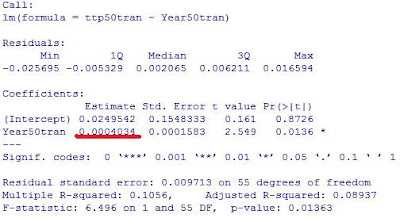
I then fit a new model of Xtransformed verus Ytransformed. The D-W statistic was 1.89 with a p value of .58 and an estimated rho of .05, thus removing the serial correlation. A summary of this model:

With such a poor fitting model (R^2 of .1056) the data does not really explain anything. If I were going to make an inference I would point out the underlined value of .0004034 (b1). The regression coeffecient for X for the transformed model will remain the same when the model is tranformed back to Y = b1*X + b0. So over the 57 years of data, 57*b1 = 2.3% increase in the Top Tenth Percentile FT%. This is really stretching the model but there may be a slight increase (2.3% over 57 years) among the best FT shooters.

More Poker Odds

I decided to finish up the poker post I had earlier. After I had calculated a few probabilities, I found a wikipedia site which covers the topic in a much more thorough manner. Last post I calculated the odds of having these starting hands: a pair (5.9%), suited connectors (3.9%), two cards both a 10 or higher (14.3%), and or of having any of these hands (20.6%).

How do these hands relate to the starting hands the other people at the table have? Using the binomial distribution and the hypergeometric distribution, I came up with this table:

The first column is the number of people at the table who have that hand, assuming that there are 10 people at the table. The Pair column says that the probability of exactly two people having a pair is 9.6%. The Ace column says that about 86.7% of the time at least one ace is dealt to the table and about 50% (34.8+13.5+1.8) of the time two or more aces are dealt to the table. So having an ace 2 for a starting hand means that it is about even odds that you do not have the best hand at the table with an ace in it.

The most useful part of the wikipedia page is the section detailing the approximation of hitting outs. Say that you have two spades and the flop gives you two more spades. That leaves 9 more spades in the deck or 9 outs to get a flush. Simply times the number of outs by 4 to get the odds of getting a flush by the river. 4*9 = 36 so 36% chance. This is an approximation with the actual probability being 34.96%. For 10 or more outs after the flop the formula is 3x+9 with x being the number of outs. The approximation on the turn is 2x (or the better approximation of 2x+(2x/10)). Pretty useful and gives you a handy way of calculating pot odds during a hand. 

Before the flop what are the odds of improving the starting hands that I mentioned above? For a pair there is roughly a 11.5% chance of getting three of a kind on the flop, 15% by the turn, and 18.5% by the turn. Chance of four of a kind is .24%, .49%, and .82% respectively. If you have two cards of the same suit it is about a .8% chance of getting a flush on the flop, 2.8% of getting it by the turn, and 5.8% of getting it by the river. The odds of getting a straight or pairing one of your cards can be found using the post-flop approximations.

Some Numbers from the 2008 Olympics

During the opening ceremonies, the US broadcast displayed a graphic with the size of the delegation and population of the country. I wondered what the correlation was between population and the number of athletes competing and what other variables might influence the delegation size. In addition to population GDP, climate, and some metric measuring civil rights for women might also explain delegation size. When I went to research this I had trouble finding the country and delegate data. What I did find was a list of all the athletes online. I turned the data into an excel file and played around a little with the data. The file can be downloaded here if anyone wants it. It is a .csv, which makes it easy to inport and analyze with R.

I created some pivot tables in Excel. It is possible to do similar things in R with the tapply() function but Excel makes pivot tables so easy to create and alter I did not bother. I uploaded them to a Google spreadsheet and embedded a few of them at the bottom of this post. The rest of the data I mainly found using R. There are 204 countries competing in this Olympics. The largest delegation belongs to the United States, with 618 athletes. 10 countries have one athlete competing: Arba, Belize, Burundi, Central Africa Republic, Dominica, Gabon, Niger, and Nauru (which was featured in a surreal This American Life episode). The mean delegation size is 49.24 athletes. Surprisingly, the median delegation size was only 9. Roughly half the countries send 9 or fewer athletes. Random fact: Only 27 of the 204 delegations have more women competing than men. Which two countries have the largest female-positive (ie more women than men) delegation?

Another column of data on the offical site listed the disciplines (sports) which athletes compete in. There are 38 discipline classifications. The most competed in discipline is Athletics (Track & Field I would guess) with 1943 competitors. Cycling BMX is the smallest event with only 24 competitors. The median and mean are 182.5 (between Baseball and Table Tennis) and 264 respectively. Random fact: there are five sports that are specific to only one gender. Which ones are they?

A little manipulation with R turned the Date of Birth data into Year of Birth and then into an 'age estimate' where I took 2008 and subtracted Year of Birth to get current age. The oldest athlete is Hoketsu Hiroshi, a 67 year-old man representing Japan in Equestrian. The youngest competitor is 12 year-old swimmer Antoinette Joyce Guedia Mouafo from Cameroon. The Median and Mean ages estimates are 26 and 26.37 years. The Random Fact was going to be the average oldest and youngest delegation, but Excel started acting up and I was a bit tired to do more R (date modification can be tricky). There is plenty to explore in this data. Let me know if you find anything neat in the above file and don't be afraid to add more columns of data.

Answers: Norway and Sweden; baseball, softball, boxing, synchronised swimming, rhythmic gymnastics